Acoustics

Introduction

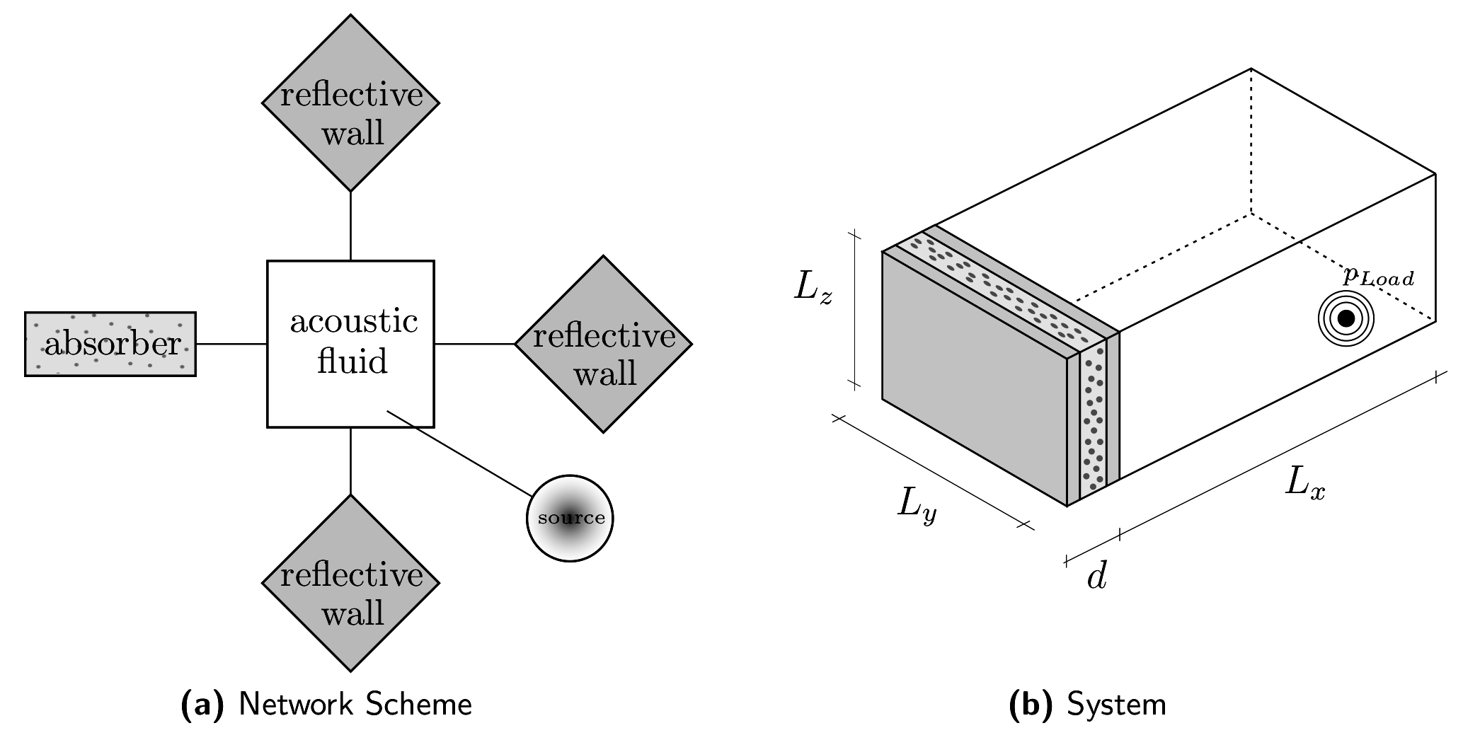
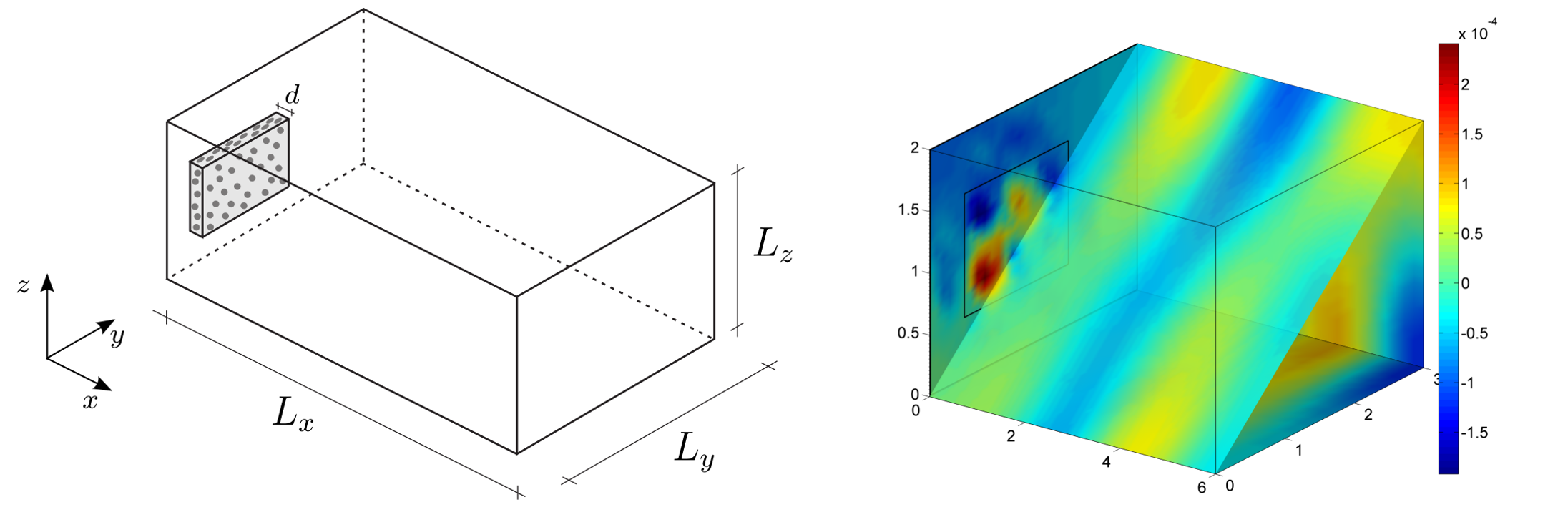
In many different fields of engineering, like automotive or civil engineering, room acoustical tasks are of interest. Sound fields have to be predicted in order to design the acoustic cavity by placing acoustic elements like reflectors or absorbers (passive absorbers or plate resonators) into the room. Hence, it is desirable to use models for the Fluid Structure Interaction (FSI) where passive absorbers or plate resonators can be considered with their specific characteristics depending on the sound wave's angle of incidence (figure 1).

Figure 1: FSI-problem (network scheme and system sketch)

In order to reduce the number of degrees of freedom and thus the numerical effort, a model reduction method based on a Component Mode Synthesis (CMS) is applied. The acoustic cavity is modeled with Spectral Finite Elements (SFEM). The cavity boundary conditions, e.g. compound absorbers made of homogeneous plates and porous foams, are modeled using Integral Transform Methods (ITM). Therefore the differential equations of motion are established for the individual components, where the Lamé Equation is used for homogenous and the Theory of Porous Media (TPM) for porous materials. These equations are solved in the wavenumber-frequency domain after applying a Fourier Transformation. The results (wavenumber dependent impedances) for the absorptive structure are coupled with the acoustic cavity adding interface coupling modes for the fluid and applying Hamilton's principle, considering the velocity of both components to coincide as a constraint at the interface.

Coupling Fluid and Substructures

Equilibrium is established using Hamilton's principle, where the subsystems arecoupled with the Lagrange Mulitplier Method.

$$\int_{t_1}^{t_2}\delta \Big( L_A(t)+L_{BC}(t,Z)+\mathbf(R)^{T}\lambda(t)\Big)+\delta W_{BC}^{nc}(t,Z) +\delta W_{Load}^{nc}(t)=0$$

With the help of a Ritz Approach the variational problem is reduced to an extremum problem.

$$\mathbf{v}_A(\mathbf{x},t)=\displaystyle\sum_{m} \mathbf{v}_{m}^{N}(\mathbf{x}) \Big(\mathcal{A}_m e^{i\Omega t} +\bar{\mathcal{A}}_m e^{i\Omega t}\Big) \displaystyle\sum_n \mathbf{v}_n^{C}(\mathbf{x}) \Big(\mathcal{B}_n e^{i\Omega t} +\bar{\mathcal{B}}_n e^{i\Omega t}\Big) $$

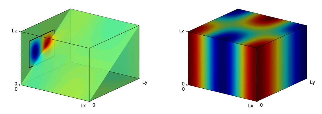
In the scope of the CMS normal modes and coupling modes, which are computed with the SFEM, are applied (figure 2). The Lagrangian of the acoustic fluid can be computed directly from these modes:

$$L_A(t)=T_A(t)-U_A(t)\ \ \ \ \ T_A(t)=\frac{\rho_A}{2} \displaystyle\int\limits_V \lvert \mathbf{V}_{A}(\mathbf{x},t)\rvert ^{2}dV \ \ \ \ U_A(t)=\frac{1}{2\rho_A c_a^{2}}\int\limits_V \lvert p_A(\mathbf{x},t)\rvert^2 dV $$

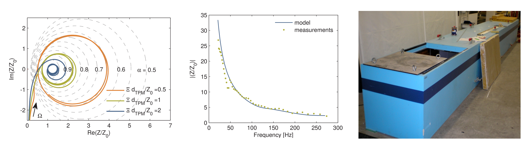
For the absorber the Lagrangian (as well as the virtual work due to dissipation) is obtained from the wavenumber- and frequency-dependent impedances as well as from the Fourier coefficients of the trial function.

$$\int \limits_0^{T} L_{BC} dt = \frac{T}{\Omega} L_y L_z \begin{bmatrix} \displaystyle\sum_n\mathcal{C}_n\bar{\mathcal{C}} \displaystyle\sum_r\displaystyle\sum_s \text{Im} \big(Z(r,s,\Omega)\big) \lvert E_{nrs}\rvert^{2}\end{bmatrix}$$

$$\int\limits_{0}^{T}\delta W_{BC} dt =-\frac{T}{i\Omega}L_y L_z \displaystyle\sum_n\big( \bar{\mathcal{C}}_n \delta \mathcal{C}_n -\mathcal{C}_n \delta \bar{\mathcal{C}}_n\big) \displaystyle\sum_r \sum\limits_s \text{Re}\big(Z(r,s,\Omega)\big) \lvert E_{nrs} \rvert ^{2}$$

Figure 2: CMS - normal modes and coupling modes

Model for Absorptive Boundaries

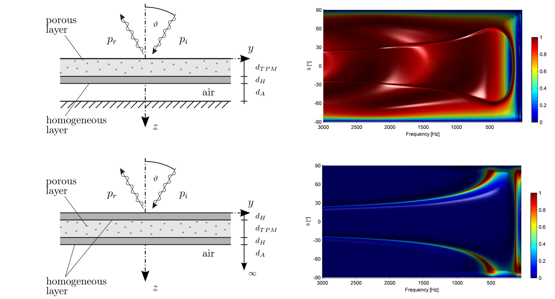
Compound absorbers, consisting of porous and elastic layers are modeled efficiently with the help of the ITM. The equations of motion, which are sketched for the porous foam exemplarily,

$$\begin{align*} -n_G \ \text{grad}p + \big( \tilde{\lambda}_S + \mu_S \big) \text{grad} \ \text{div} \ \mathbf{u}_S+ \mu_s \ \text{div} \ \text{grad} \ {\mathbf{u}_S}+ S_G(\mathbf{v}_G-\mathbf{v}_S)&= \rho_S \mathbf{a}_S \\ -n_G \ \text{grad}\ p-S_G(\mathbf{v}_G+\mathbf{v}_S)&= \rho_G\mathbf{a}_G \end{align*} $$

$$\frac{n_G}{R\theta} \ \frac{\partial p}{\partial t} +\rho_{GR}\ n_G \ \text{div}(\mathbf{v}_G) +\rho_{GR}\ n_S \ \text{div}(\mathbf{v}_S)$$

are established for each material and solved in the Fourier domain after applying a Helmholtz decomposition considering of the boundary conditions at the interfaces between the individual layers in order to compute wavenumber and frequency-dependent impedances and absorption ratios.

Figure 3: Plane-wave impedances (numerical results and verification with measurements)

Figure 4: Wavenumber and frequency-dependent absorption ratio (trace matching characteristics)

Numerical Results for the FSI-Problem

The method is applied to a rectangular geometry (6m × 3m × 2m), which is modeled with 288 spectral finite elements. In the CMS 50 normal and 6 couplingmodes are considered. A pressure source is applied at x = 0.5 m, y = 1.3 m andz = 0.9 m. It is oscillating with a frequency of 122 Hz. The absorptive boundary condition is modeled as layer of melamine foam with a thickness of 7.2 cm.

The sound pressure field is computed and visualized in figure 5.

Figure 5: 3d FSI example - sound pressure field in an acoustic cavity with a porous absorber

Contact

Quirin Aumann