Augmented Beam Elements

Introduction

In past decades, various formulations of beam elements were derived with the aim of efficiency of calculation, stability and accuracy of computation. Nevertheless, this accuracy holds always with respect to the assumptions underlying the beam theory, such as plane cross-sections and consequently constant shear stress across a section. For some practical applications like bridge design, these restrictions are not acceptable, and thus such beam-like structures typically are modelled using solid Finite Elements. The drawbacks are the “loss” of comprehensible quantities like the internal forces and a high modelling effort especially at the supports and considerably high computation time.

Description of the Method of Unit Deflection Shapes

Fig.1: Eigenmodes of the Cross Section as a Plate in Bending Action

Fig.2: Eigenmodes of the Cross Section as a Plate in Membrane Action

The idea of this work is to keep the beam element fashioned modelling of structures but enhance the solution space such that arbitrary, reasonable deflection shapes of the cross section can be covered. The concept is in analogy with the concept of warping torsion of beam elements. New degrees of freedom are introduced at the nodes which correspond to the contribution of a certain unit deflection shape at the node. The unit deflection shapes can contain either out of plane or in plane deflections which are defined on the basis of a 2D finite element mesh of the cross section. The shapes for the unit deflection modes are obtained with various procedures making use of the Finite Element mesh of the cross section:

Eigenmodes of an Infinite Waveguide Structure

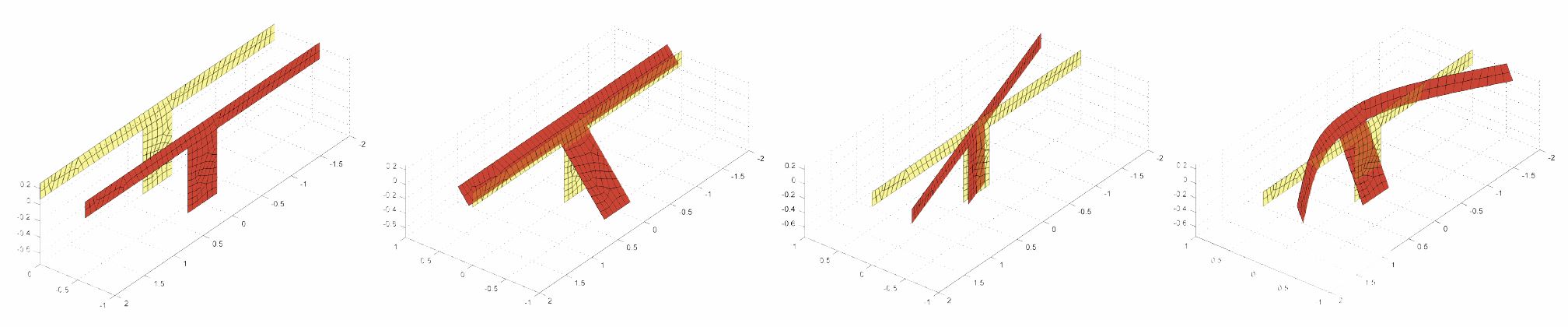
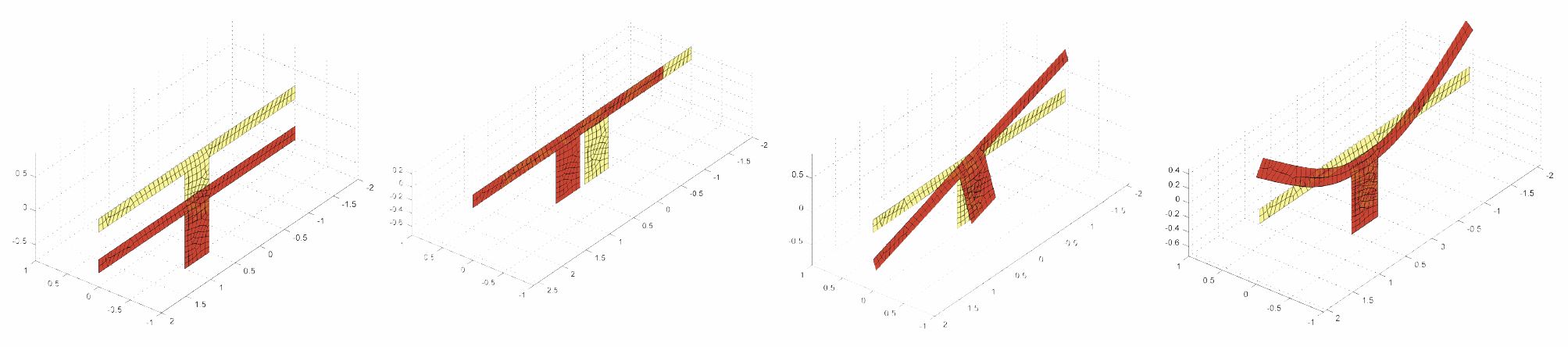
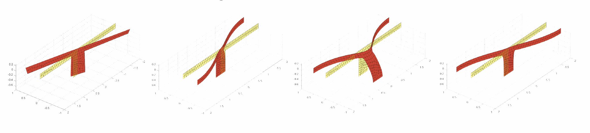
Further unit deflection shapes are gained by solving an eigenvalue problem for an infinite waveguide structure with the considered cross section in the Fourier transformed frequency - wavenumber domain for a fixed frequency. After the inverse transformation the unit deflection shapes are gained for example for a rectangle cross section:

For low frequencies (here: 10 Hz) the eigenvalues occur for the waves of a classical beam: longitudinal compression, torsion and bending. Each mode occurs twice - for both propagation directions (positive and negative x-direction).

Orthogonalization

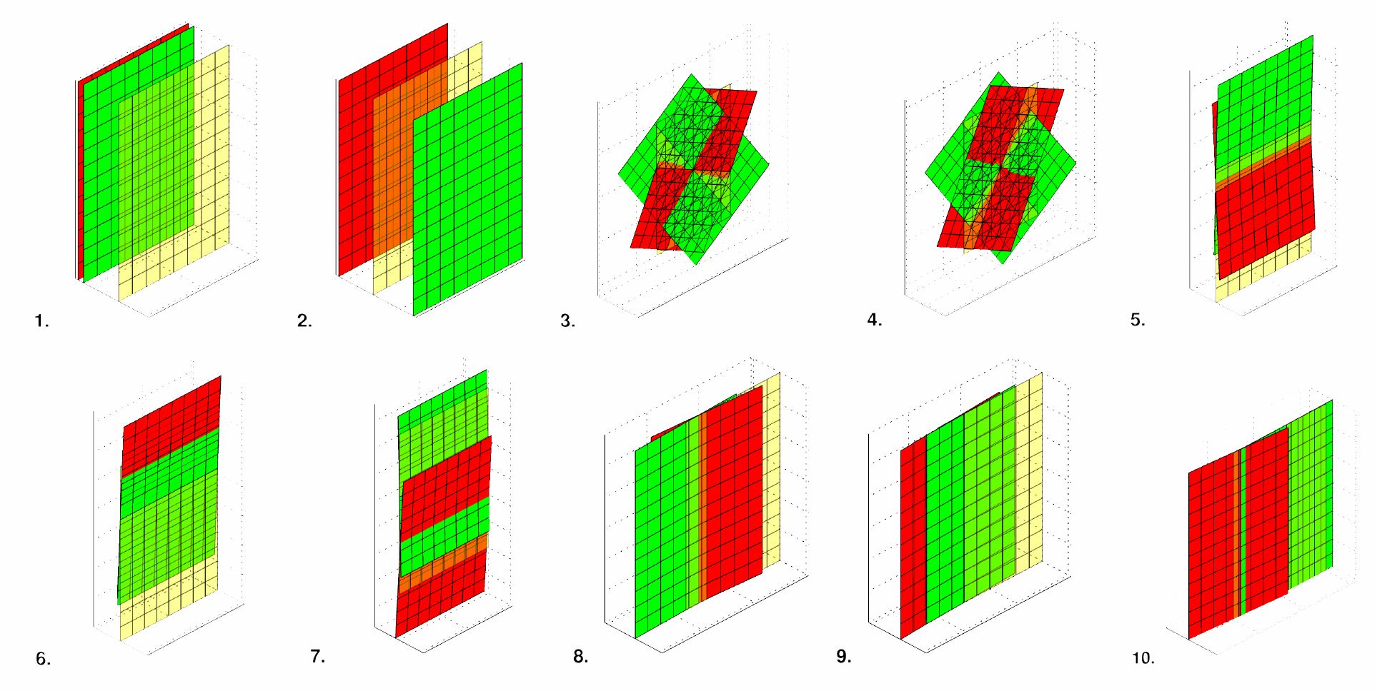
Provided that the mode shapes are linearly independent further orthogonalization is not mandatory from a computational or numerical point of view. Nevertheless, orthogonalization is necessary to allow for comprehensive values like moment, shear force or normal force and the ability to introduce comprehensive boundary conditions like for example a simple support. Additionally, it allows for comprehensive loading like transverse loads or line moments. The orthogonalization is organized hierarchically. From every further deflection shape the contained components of all preceding deflection shapes are subtracted by the following scheme:

$$\mathbf{\psi}_{i, \text{ortho}} = \mathbf{\psi}_{i} - \sum\limits_{k=1}^{i-1} \frac{{\mathbf{\psi}_{i}}^T \cdot \mathbf{A} \cdot \mathbf{\psi}_{k}}{{\mathbf{\psi}_{i}}^T \cdot \mathbf{A} \cdot \mathbf{\psi}_{i}} \cdot \mathbf{\psi}_{k}$$

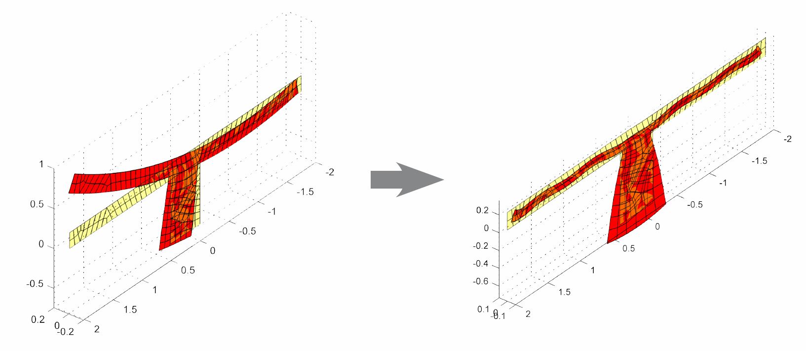
Fig.5: Orthogonalisation of a Unit Deflection Shape

Through the orthogonalization the unit deflections change their shape:

Beam Element and System Stiffness Matrix

The system unknowns are the scaling factors of these deflection shapes. The number of considered shapes can be chosen according to the requirements on accuracy and the expected deflection shape. “Higher modes” can be neglected and thus an adaptive and efficient solution scheme is obtained. The structure of the problem with its comparably small number of system unknowns is solved very fast. The setup of the system stiffness- and mass matrices and the computation of stresses (postprocessing) is computationally expensive but well suitable for parallelization. This property opens the gate for massive performance gains since also modern core architectures can be made use of in an optimal way. $$\mathbf{\underline{K}}_{\text{beam}}=\mathbf{N}^T\cdot\mathbf{K}_{\text{bricks}}$$ With $$\mathbf{N}=\begin{bmatrix} \mathbf{\psi}_1&\mathbf{0}&\mathbf{\psi}_2& \mathbf{0}&\cdots&\mathbf{\psi}_{n_\text{modes}}&\mathbf{0}\\ \mathbf{0}&\mathbf{\psi}_1&\mathbf{0}&\mathbf{\psi}_2&\cdots&\mathbf{0}&\mathbf{\psi}_{n_\text{modes}}\end{bmatrix}$$

Examples

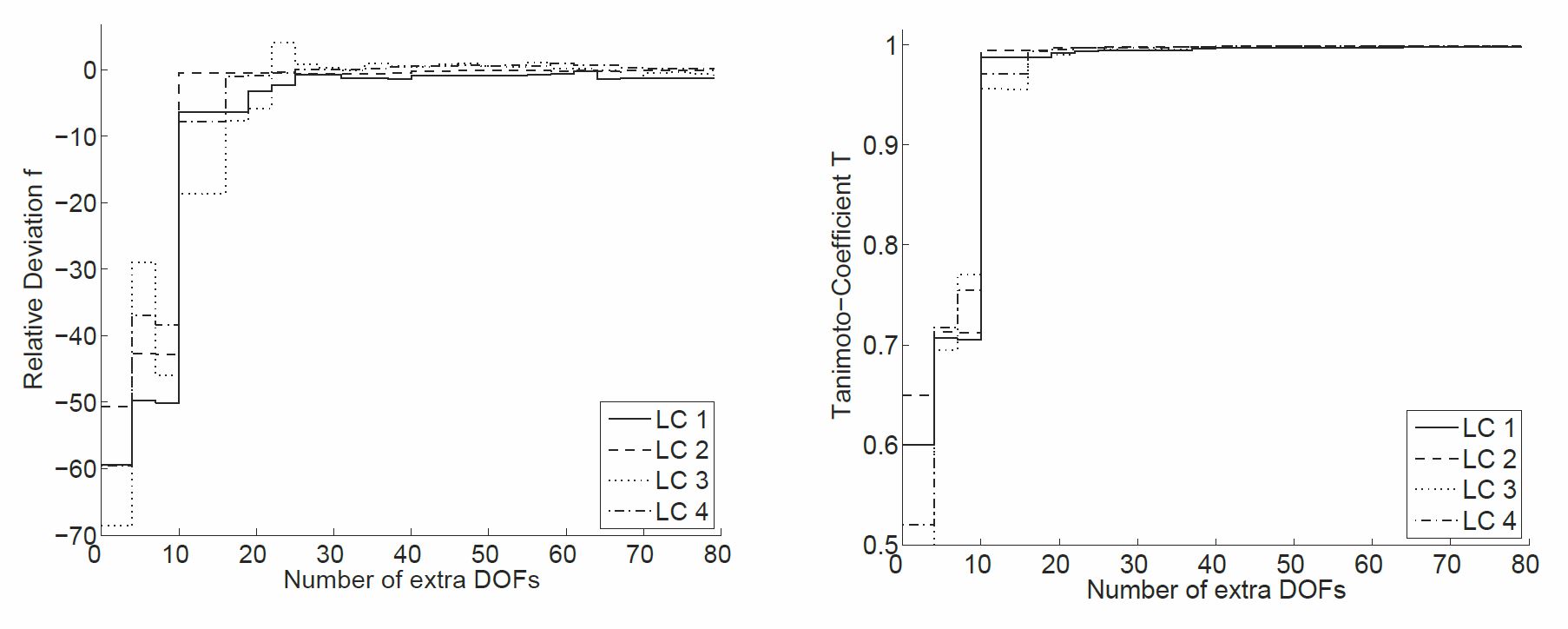
The method was evaluated for different systems applying different load cases using different combinations of the shown types of deflection shapes. All results showed a quick convergence. The following graphs show the evaluation for an example of a two span beam under different load cases. The reference calculation was a Finite Element volume model with more than 200 DOFs per section.

Fig.6: Convergence of the described method with increasing number of considered degrees of freedom

Contact

Axel Greim, M.Sc.